Introduction to PIC

Introduction to PIC

A plasma is composed of a vast number of charged particles that interact with each other through electromagnetic fields in complex, long-range, collective interactions. Plasma behavior is highly complex, forming a truly non-local, non-equilibrium, nonlinear system (as noted in Taccogna, 2018). The core mission of the Particle-in-Cell (PIC) method is to provide a computationally tractable approach that can still capture as many plasma processes as possible.

Compared to other (potential) computational methods, PIC has irreplaceable advantages:

• Compared to fluid models: In fluid models, plasma is treated as a continuous fluid (e.g., magnetohydrodynamics, MHD). Fluid models are well-suited for describing large-scale, low-frequency phenomena. However, when kinetic effects become important, fluid models break down. These effects include: non-Maxwellian velocity distributions (e.g., particle beams), wave-particle interactions (such as Landau damping), and behavior near boundaries (sheaths).

• Compared to directly solving the N-body problem: Directly simulating the "N-body" interactions among trillions of real particles is computationally absolutely infeasible. Handling certain electromagnetic field boundary conditions would also become difficult.

• Compared to directly solving kinetic equations: The Vlasov equation, which describes the kinetic behavior of plasmas, is a partial differential equation defined in a six-dimensional phase space (3 spatial dimensions + 3 velocity dimensions). Directly solving this equation on such a high-dimensional grid (known as the Eulerian approach or Vlasov simulation) is extremely computationally expensive. This approach is not entirely infeasible, but its range of applicability remains quite limited to date.

Although the computational cost is still high, PIC has become a practical and reliable method for simulating plasma behavior.

The Vlasov-Poisson System

The Vlasov-Poisson system is the most fundamental model for describing the kinetic behavior of plasmas. It is the classic starting point for PIC simulations, particularly suited for studying electrostatic phenomena.

In three-dimensional space, this system consists of two equations:

1. Vlasov Equation: Describes how the particle distribution function \(f_s\) (\(s\) represents different particle species, such as electrons \(e\) and ions \(i\)) evolves in a self-consistent electric field \(\mathbf{E}\). It is a 6-dimensional partial differential equation:

\[\frac{\partial f_s}{\partial t} + \mathbf{v} \cdot \nabla_{\mathbf{x}} f_s + \frac{q_s}{m_s}\mathbf{E} \cdot \nabla_{\mathbf{v}} f_s = 0 \tag{1}\]

1. Poisson's Equation: Describes how the electric field \(\mathbf{E}\) is generated by the spatial distribution of all particles (i.e., the charge density \(\rho\)). Under the electrostatic assumption, the electric field \(\mathbf{E}\) can be expressed as the gradient of the electric potential \(\phi\) (\(\mathbf{E} = -\nabla \phi\)), yielding Poisson's equation. It is a 3-dimensional partial differential equation:

\[\nabla^2 \phi = -\frac{\rho}{\epsilon_0} \tag{2}\]

These two equations are coupled through the charge density \(\rho\). \(\rho\) is obtained by integrating the distribution functions \(f_s\) of all particle species:

\[\rho(\mathbf{x}, t) = \sum_s q_s \int f_s(\mathbf{x}, \mathbf{v}, t) d\mathbf{v} \tag{3}\]

These three equations represent the three fundamental elements for describing plasma from a kinetic perspective:

• The distribution function evolves over time under a given electric field;
• The spatial distribution of free charge determines the spatial distribution of the electric field;
• The velocity-space integral of the distribution function determines the charge distribution.

Replacing Poisson's equation with Maxwell's equations yields a more physically complete model; however, for many problems, Poisson's equation suffices.

Two Perspectives: Macro-Particles and Characteristics

A plasma consists of a large number of interacting microscopic charged particles. As an N-body system, the enormous N (typically far exceeding \(10^{12}\)) directly renders computation infeasible. In PIC, we do not (typically) track every individual real electron or ion. Instead, it tracks macro-particles (also called super-particles): a single macro-particle represents a large group of real particles with similar positions and velocities (e.g., \(10^6\) or \(10^{10}\) electrons). Imagine replacing the particles in the original plasma with a much smaller number of macro-particles that conserve charge and mass — most physical phenomena should remain unchanged.

We assume that this macro-particle possesses the total charge and total mass of the group of particles it represents, and is located at their average position \(\mathbf{x}_j\). We then compute the motion of this macro-particle using Newton's second law:

\[\frac{d\mathbf{x}_j}{dt} = \mathbf{v}_j\]

\[\frac{d\mathbf{v}_j}{dt} = \frac{q_j}{m_j} (\mathbf{E}(\mathbf{x}_j) + \mathbf{v}_j \times \mathbf{B}(\mathbf{x}_j))\]

PIC can thus be viewed as actually solving for the evolution of this macro-particle system. By tracking the motion of each macro-particle, we can compute the evolution of the plasma as a whole.

The above describes an intuitive way to understand PIC. In theoretical analysis, another perspective is equally meaningful: recall the Vlasov equation, which describes the evolution of the distribution function \(f(\mathbf{x}, \mathbf{v}, t)\) in six-dimensional phase space. Taking the simplest collisionless, electrostatic case as an example:

\[\frac{\partial f}{\partial t} + \mathbf{v} \cdot \nabla_{\mathbf{x}} f + \frac{q}{m}\mathbf{E} \cdot \nabla_{\mathbf{v}} f = 0\]

This is a partial differential equation. A classical method for solving it is the Method of Characteristics. This method tells us that along a particular phase-space trajectory (i.e., a "characteristic"), the value of the distribution function \(f\) remains constant. These characteristics are defined by a set of ordinary differential equations:

\[\frac{d\mathbf{x^*}}{dt} = \mathbf{v^*}\]

\[\frac{d\mathbf{v^*}}{dt} = \frac{q}{m}\mathbf{E}(\mathbf{x^*}, t)\]

Along the trajectory \((\mathbf{x^*},\mathbf{v^*})\), we have:

\[f(\mathbf{x^*}_{t=0}, \mathbf{v^*}_{t=0}, t=0) = f(\mathbf{x^*}_{t=\tau}, \mathbf{v^*}_{t=\tau}, t=\tau)\]

Therefore, if we sample the initial distribution \(f_{t=0}\) as a set of points in 6-dimensional phase space, and use the positions and velocities of these points as initial conditions for the characteristic equations, then after advancing these points along the characteristics by \(\Delta t\), they constitute a sampling of \(f_{t=\Delta t}\)! That is:

\[ f_0 \xrightarrow{sample} {\left\{(\mathbf{x^*},\mathbf{v^*})_{t=0}\right\}} \xrightarrow{push} {\left\{(\mathbf{x^*},\mathbf{v^*})_{t=\Delta t}\right\}} \xrightarrow{sample\ representation} f_{\Delta t} \]

Thus, by repeatedly pushing a set of points in phase space along characteristics, we can express the evolution of the distribution function in an indirect manner. Note that the equations satisfied by the characteristics are exactly the same as the equations of motion we use to advance macro-particles. From this perspective, each macro-particle in PIC is a sample of the phase-space distribution, and the characteristic equations it satisfies are precisely the equations of motion for charged particles. This is why PIC is in fact also a kinetic simulation method.

Comparing with the Vlasov-Poisson system we wish to solve, PIC provides a concrete method for solving the Vlasov equation. Specifically:

• Discretization of the distribution function: Each charged particle species is discretized into a set of macro-particles.
• Update of the distribution function: Updating the macro-particles according to the equations of motion of charged particles simulates the evolution of the distribution function.

Particle-Field Coupling

The discretized solution of Poisson's equation can be achieved using finite difference, finite volume, or finite element methods, which will not be elaborated here. PIC also needs to address the coupling between the Vlasov equation and Poisson's equation. In the standard PIC method, this coupling is implemented by alternately solving the two equations, involving the following steps:

• Particle push (Vlasov): Interpolate the electromagnetic field at each macro-particle's position, and update all macro-particles' positions \(\mathbf{x}_j\) and velocities \(\mathbf{v}_j\) according to Newton's second law.
• Charge assignment (integration): Distribute the charge \(q_j\) of all macro-particles onto the spatial grid nodes, constructing the gridded charge density \(\rho\). This is the numerical implementation of equation (3).
• Field solve (Poisson): Solve Poisson's equation \(\nabla^2 \phi = -\rho / \epsilon_0\) on the grid to obtain the gridded electric potential \(\phi\). Then compute the electric field on the grid as \(\mathbf{E} = -\nabla \phi\).

By cycling through these steps, the evolution of the plasma can be simulated. However, there are still two problems to resolve:

• How to obtain the local electric field based on the electric field computed in the previous step and the particle positions?
• How to obtain the spatial distribution of charge density based on particle positions?

In standard PIC on structured grids, the answer to both questions is the area weighting method (Cloud-in-Cell, CIC), as shown in the following figure:

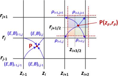
That is, we consider particles to have the same shape as the grid, and the overlap between each cell and the particle area determines the weight contributed by that cell.

It should be emphasized that the interpolation scheme is not unique, and it has a significant impact on the overall numerical properties of the PIC method. This remains an important area of ongoing research in PIC methods.