big_bang

Big Bang

This document walks through the development of a 2D electrostatic PIC (Particle-In-Cell) example.

The example places a small cluster of same-sign charged particles in a square domain [-1, 1] x [-1, 1]. The particles are initially concentrated near the origin, then repel each other under the self-consistent electric field and expand outward; particles reaching the boundary are absorbed. This example covers the main workflow of electrostatic PIC, but does not include collisions, magnetic fields, or complex geometric boundaries.

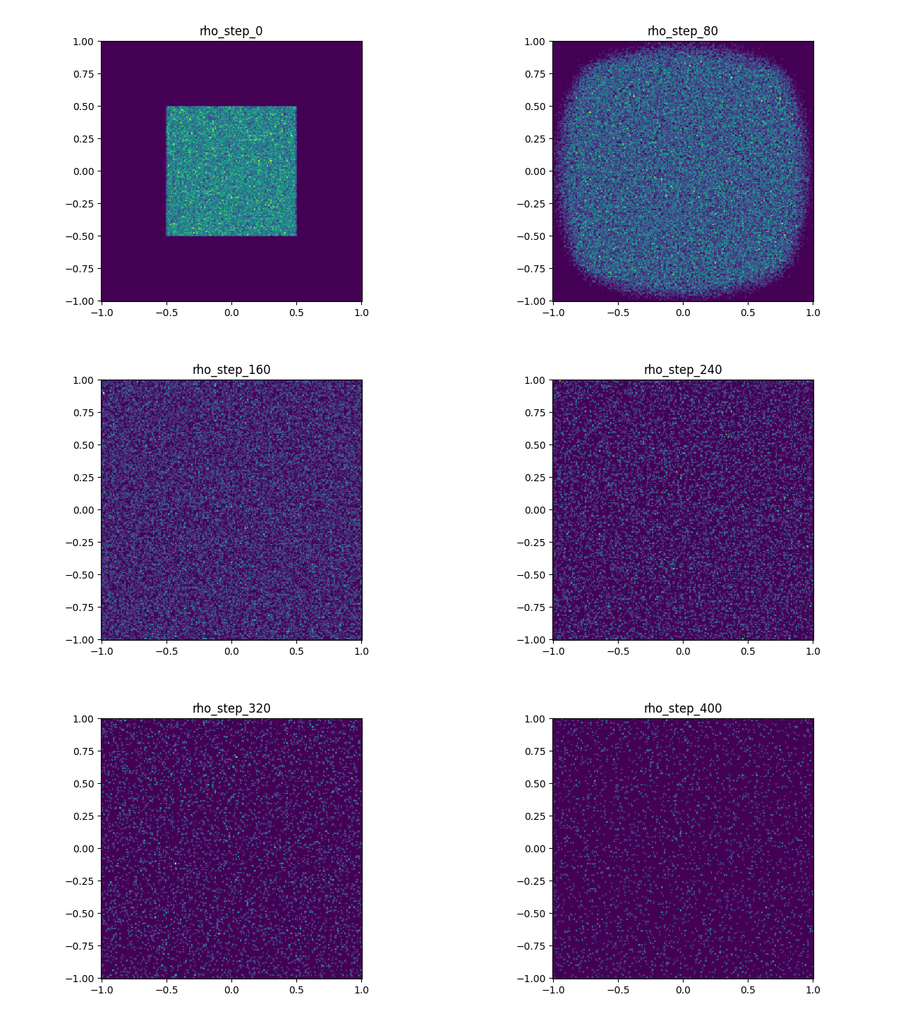
Modules, features, and typical usage covered:

• Particle definition and particle containers
• Particle-field interaction
• Poisson equation solving

Preparation

Create a new file big_bang.cpp under example/big_bang/, then modify it step by step according to each stage. example/big_bang/stage_1.cpp through stage_6.cpp are reference answers at the end of each stage, for comparing with your own code; they are not programs you must run.

It is recommended to enter the example directory from the project root and load the build environment:

cd example/big_bang
source ../../env_load.sh

There may be leftover .plt, .png, or .gif files in output/. You can manually clear output/ first.

Stage 1: Create the Grid and Fields

In big_bang.cpp, first include the necessary headers and use namespace psum::prelude:

#include <iostream>
#include <sycl/sycl.hpp>
#include <Eigen/Core>
#include <psum/psum.hpp>
using namespace std;
using namespace psum::prelude;

Add the particle type definition:

using Particle = tagged_struct<
    tag_bind<property::position, Eigen::RowVector2d>,  // 2D position
    tag_bind<property::velocity, Eigen::RowVector2d>,  // 2D velocity
    tag_bind<property::charge, double>,                // charge
    tag_bind<property::mass, double>                 // particle mass
>;

Add the grid definition in the main function:

int main() {
    grid2D grid({-1.0, -1.0}, {1.0, 1.0}, {256, 256});
    sycl::queue q{sycl::default_selector_v};

    // You can see the device info
    cout << "device: " << q.get_device().get_info<sycl::info::device::name>() << endl;

    // Node fields for storing electric potential and charge density (device-side, usable in kernels)
    node_field2D<double> phi(q, grid);      // electric potential
    node_field2D<double> rho(q, grid);      // charge density

    return 0;
}

Write the makefile:

-include ../../config.mk

INCLUDES = -I ../../include -I ../../src

big_bang: big_bang.cpp
    $(ACPP) $(COMMON_FLAGS) $(INCLUDES) -o bb big_bang.cpp $(LIBS) $(LDFLAGS)
    ./bb

(These commands already exist in example/big_bang/makefile, just uncomment them.)

For subsequent stages, compile and run the same way:

make big_bang

Before compiling, make sure you have sourced env_load.sh from the project root, then run make big_bang. If you see make: acpp: No such file or directory, it usually means you haven't run source ../../env_load.sh yet, or the dependencies/installation were not successful.

After a successful run, you should see the device info printed, for example AdaptiveCpp OpenMP host device (if your machine has a GPU, it may show the GPU model instead). On the first run, AdaptiveCpp may print kernel cache warnings; these are typically just JIT compilation notices, not program failures.

What you need to know at this stage:

• Particle defines what attributes a particle has.
• grid2D defines the 2D computational domain and grid resolution.
• node_field2D is a field defined on grid nodes, used here for electric potential phi and charge density rho.

The code state at the end of this stage can be found in example/big_bang/stage_1.cpp.

Step 2: Add Particle Container and Initialize Particles and Charge Deposition

Continue modifying big_bang.cpp from Stage 1:

• Add ParticleGroup after the Particle definition.
• Add make_particles and deposit_charge before main.
• In main, create the particle container, initialize particles, deposit charge, then output output/initial_rho.plt.
• Modify the makefile to create output/ first, then run the program and generate images.

After Particle, define particle_group as the particle container:

using ParticleGroup = particle_group<Particle, pos_x_nan_is_invalid>;

The pos_x_nan_is_invalid here will be used later in the boundary absorption stage: when a particle is marked as invalid, particle_group iteration will automatically skip it.

The particle initialization function takes ParticleGroup& directly, generates a host-side vector<Particle> inside the function, and inserts all particles into the particle group at once:

void make_particles(size_t count, ParticleGroup& particles) {
    rander R;
    vector<Particle> particle_vec(count);
    for (auto& p : particle_vec) {
        get<property::position>(p) = {R() - 0.5, R() - 0.5};
        auto rand_vec = RandFunction3D::RandV_Maxwell(R, 100000, 2.18e-25);
        get<property::velocity>(p) = {rand_vec.x(), rand_vec.y()};
        get<property::charge>(p) = 1.602e-19 * 1e7;
        get<property::mass>(p) = 2.18e-25 * 1e7;
    }
    particles.insert(particle_vec);
}

The position here is uniformly distributed over [-0.5, 0.5] x [-0.5, 0.5]. Velocity is generated using the Maxwell distribution via RandFunction3D::RandV_Maxwell from PSuM's random utilities, then the x/y components are taken as 2D velocities. Charge and mass are both multiplied by 1e7, representing many real particles (macro-particles).

Next, add the charge deposition function:

void deposit_charge(ParticleGroup& particles, node_field2D<double>& rho) {
    rho.setZero();
    double cell_area = rho.getGrid().del<0>() * rho.getGrid().del<1>();
    particles.for_each([&](sycl::handler& h) {
        auto rho_acc = rho.get_access(h);
        return [=](Particle& p) {
            add_back(
                get<property::position>(p),
                get<property::charge>(p) / cell_area,
                rho_acc
            );
        };
    });
}

Note that cell_area is obtained directly from rho.getGrid(), so deposit_charge doesn't need additional grid parameters. rho.setZero() clears the previous deposition result, and add_back adds particle charge to grid nodes with interpolation weights.

In main, add:

ParticleGroup particles(q);
make_particles(100000, particles);
deposit_charge(particles, rho);
rho.plot("output/initial_rho.plt", "rho", 0.0);

Adjust the makefile:

big_bang: big_bang.cpp
    $(ACPP) $(COMMON_FLAGS) $(INCLUDES) -o bb big_bang.cpp $(LIBS) $(LDFLAGS)
    mkdir -p output # create output directory
    ./bb
    python3 ../pltview.py output/initial_rho.plt # convert the generated plt file to png

After a successful run, you should see output/initial_rho.plt and the generated output/initial_rho.png. If .png is not generated, first check whether python3 ../pltview.py output/initial_rho.plt was executed, and whether the current directory is example/big_bang/.

What you need to know at this stage:

• ParticleGroup is a container that holds many particles.
• make_particles first generates particles on the host side, then inserts them into the container all at once.
• deposit_charge distributes particle charge to grid nodes with interpolation weights.

The code state at the end of this stage can be found in example/big_bang/stage_2.cpp.

Step 3: Add Particle Motion and Boundary Conditions

Continue modifying big_bang.cpp from Stage 2:

• Add move_particles after deposit_charge.
• Change the "deposit once and output" code in main to a time loop.
• Modify the makefile to combine rho_step_*.plt files into an animation.

At this stage, we don't add the Poisson solver yet, so phi is still a zero field; however, we still write the full PIC push logic that derives the electric field from phi. This way, in the next stage we only need to make phi the potential computed by the solver, without changing the particle push function.

Add the particle motion function after deposit_charge:

void move_particles(ParticleGroup& particles, node_field2D<double>& phi, double dt) {
    particles.for_each([&](sycl::handler& h) {
        auto phi_acc = phi.get_access(h);
        return [=](Particle& p) {
            auto& position = get<property::position>(p);
            auto& velocity = get<property::velocity>(p);

            auto grad_phi = interp_diff(position, phi_acc);
            Eigen::RowVector2d electric_field(-grad_phi[0], -grad_phi[1]);
            velocity += electric_field * get<property::charge>(p) / get<property::mass>(p) * dt;
            position += velocity * dt;

            if (!phi_acc.getGrid().inGrid(position)) {
                ParticleGroup::validator::make_invalid(p);
            }
        };
    });
}

Here interp_diff(position, phi_acc) returns the gradient of the potential, and the electric field is -grad(phi). Currently phi is zero, so the electric field is zero. Particles only fly with their initial Maxwell velocities. For boundary handling, ParticleGroup::validator::make_invalid(p) is used; particles marked as invalid will be skipped in subsequent particle_group iterations.

Then replace the "deposit once" part from step 2 with a time loop:

double dt = 2.0e-7;
int steps = 400;
int output_interval = 10;

for (int step = 0; step <= steps; ++step) {
    deposit_charge(particles, rho);
    if (step % output_interval == 0) {
        rho.plot("output/rho_step_" + to_string(step) + ".plt", "rho", step * dt);
        cout << "step = " << step << ", alive = " << particles.size() << endl;
    }
    move_particles(particles, phi, dt);
}

Adjust the makefile to create an animation with pltview.py after running the program:

big_bang: big_bang.cpp
    $(ACPP) $(COMMON_FLAGS) $(INCLUDES) -o bb big_bang.cpp $(LIBS) $(LDFLAGS)
    mkdir -p output
    ./bb
    python3 ../pltview.py rho_step output

python3 ../pltview.py rho_step output will search for .plt files starting with rho_step_ in output/ and combine them into an animation. After a successful run, the terminal will print step = ..., alive = ..., and generate output/rho_step.gif. Although phi is a zero field at this stage, particles will still fly with their initial Maxwell velocities, so a small number of particles will leave the boundary later.

What you need to know at this stage:

• interp_diff(position, phi_acc) computes the gradient from the potential field.
• The electric field is -grad(phi); currently phi is zero, so there is no self-consistent electric field acceleration yet.
• Particles leaving the grid are marked as invalid and will be skipped in subsequent iterations.

The code state at the end of this stage can be found in example/big_bang/stage_3.cpp.

Step 4: Add the Poisson Solver

Continue modifying big_bang.cpp from Stage 3:

• Add boundary condition utilities in the namespace section.
• After creating particles, create Poisson_solver_2d and set four Dirichlet boundaries.
• Add host-side temporary fields phi_host and rho_host.
• After each charge deposition, solve for phi, and temporarily keep if (step == 0) break; to only check the initial potential.
• The makefile compilation command adds $(USE_BACKENDS) from this stage onward.

At this stage, we replace the phi that has been zero in step 3 with the potential solved from charge density rho. To first verify the Poisson solver and potential output separately, this step exits the program after completing the rho -> phi solve and output at step 0.

First, add boundary condition utilities in the namespace section:

using namespace psum::field_solver::boundary_creator;

After creating particles, create the Poisson solver and set all four edges as fixed-value boundaries:

Poisson_solver_2d psolver;
psolver.init(
    grid,
    Poisson_solver_2d::Cartesian,
    {
        Dirichlet_line(grid, boundary_direction_2d::N) = 0,
        Dirichlet_line(grid, boundary_direction_2d::S) = 0,
        Dirichlet_line(grid, boundary_direction_2d::E) = 0,
        Dirichlet_line(grid, boundary_direction_2d::W) = 0
    }
);

The current native backend works on the host side, so you also need to prepare host-side temporary fields:

host_node_field2D<double> phi_host(grid);
host_node_field2D<double> rho_host(grid);

Then in the main loop, solve for the potential after each charge deposition:

for (int step = 0; step <= steps; ++step) {
    deposit_charge(particles, rho);
    rho_host.copy(rho.getContent().to_host());
    psolver.solve(phi_host.data(), rho_host.data());
    phi.copy(phi_host.getContent());

    if (step % output_interval == 0) {
        rho.plot("output/rho_step_" + to_string(step) + ".plt", "rho", step * dt);
        phi.plot("output/phi_step_" + to_string(step) + ".plt", "phi", step * dt);
        cout << "step = " << step << ", alive = " << particles.size() << endl;
    }
    if (step == 0) break; // temporary logic, only output initial distribution
    move_particles(particles, phi, dt);
}

Here rho_host.copy(rho.getContent().to_host()) copies device-side rho to host; psolver.solve(phi_host.data(), rho_host.data()) solves the Poisson equation; phi.copy(phi_host.getContent()) copies the host-side potential back to device-side phi.

Whether you need host-side copies depends on whether the solver backend supports device-side pointers. For GPU backends like cuda_sparselu_gpu, this step is not needed (and would cause errors).

Adjust the makefile to view the initial potential after running the program:

big_bang: big_bang.cpp
    $(ACPP) $(COMMON_FLAGS) $(INCLUDES) -o bb big_bang.cpp $(USE_BACKENDS) $(LIBS) $(LDFLAGS)
    mkdir -p output
    ./bb
    python3 ../pltview.py phi_step output

Here $(USE_BACKENDS) is added to facilitate using non-native backends later. If linking reports missing registry.o, impls.o, or other field solver backend files, it means the solver backend has not been built yet. You need to build these backend object files first according to the build documentation.

After running, you should get output/phi_step.png. This stage only outputs step 0, so pltview.py generates a single image instead of an animation. The potential distribution should be smoother than the charge distribution and reach 0 at all four boundaries. This tutorial uses the native backend by default, so the two host/device copies rho_host.copy(...) and phi.copy(...) are needed. If you switch to a GPU backend later, this code can be removed.

What you need to know at this stage:

• The Poisson solver converts charge density rho to electric potential phi.
• $(USE_BACKENDS) links the solver backend into the program.
• Here we exit at step 0 first, to separately confirm that the potential solve and output are correct.

The code state at the end of this stage can be found in example/big_bang/stage_4.cpp.

Step 5: Use the Solver-Computed Electric Field to Update Particle Positions

Continue modifying big_bang.cpp from Stage 4:

• Delete if (step == 0) break; in the main loop.
• In the makefile, generate animations for both rho_step and phi_step.

Step 4 can already compute the potential from the current particle distribution, but the program exits at step 0. There is very little to do at this stage: just remove

if (step == 0) break;

from the main loop.

Adjust the makefile to generate both charge density and potential animations after running:

big_bang: big_bang.cpp
    $(ACPP) $(COMMON_FLAGS) $(INCLUDES) -o bb big_bang.cpp $(USE_BACKENDS) $(LIBS) $(LDFLAGS)
    mkdir -p output
    ./bb
    python3 ../pltview.py rho_step output
    python3 ../pltview.py phi_step output

After running, you should see the particle cluster expand rapidly; particles reaching the boundary are marked as invalid by ParticleGroup::validator::make_invalid(p), so the alive count will decrease.

What you need to know at this stage:

• Each step first deposits rho, then solves phi, and finally pushes particles using phi.
• output/rho_step.gif shows how the charge density (corresponding to particle spatial distribution) expands.

The code state at the end of this stage can be found in example/big_bang/stage_5.cpp.

Step 6: Observe Energy Conservation

Continue modifying big_bang.cpp from Stage 5:

• Add <fstream>.
• Add kinetic_energy and field_energy after move_particles.
• In main, open output/energy.plt; create a reusable shared variable.
• After solving for phi, tally the total energy and write it to the file.
• Add python3 ../pltview.py energy output to the makefile.

Step 5 has completed the self-consistent particle push: each step first deposits rho from particles, then solves phi, and finally pushes particles with the electric field. Now we can add an energy diagnostic to observe whether the numerical process is roughly conservative before a large number of particles leave the boundary.

First add <fstream> needed for file output:

#include <fstream>

Particle kinetic energy can be directly accumulated in parallel on the particle container. Since all particles simultaneously write to the same scalar, this scalar needs to be placed in device-accessible shared memory, with atomic_add for reduction:

double kinetic_energy(ParticleGroup& particles, double* energy) {
    *energy = 0.0;
    particles.for_each([&](sycl::handler& h) {
        return [=](Particle& p) {
            const auto& velocity = get<property::velocity>(p);
            atomic_add(*energy, 0.5 * get<property::mass>(p) * velocity.squaredNorm());
        };
    });
    return *energy;
}

Field energy is the integral (accumulation) of the product of charge density and potential, which can be implemented using the for_each function provided by the field:

double field_energy(node_field2D<double>& phi, node_field2D<double>& rho, double* energy) {
    *energy = 0.0;
    double cell_area = phi.getGrid().del<0>() * phi.getGrid().del<1>();
    phi.for_each([&](sycl::handler& h) {
        auto rho_acc = rho.get_access(h);
        return [=](size_t i, double& phi_value) {
            atomic_add(*energy, 0.5 * phi_value * rho_acc(i) * cell_area);
        };
    });
    return *energy;
}

Here phi.for_each's first parameter i gives the current grid point index, and rho_acc(i) accesses the charge density at the same location.

In main, open the energy file and create a reusable shared variable:

ofstream energy_file("output/energy.plt");
energy_file << "variables=time,relative_energy" << endl;
double initial_energy = 0.0;
double* energy = shared_variable<double>(q);

energy is created only once in the main function, then passed to both the kinetic and field energy functions for reuse. Each function resets *energy to zero at the start.

In the main loop, after solving for phi, immediately tally the total energy and its relative value:

double kinetic = kinetic_energy(particles, energy);
double electric = field_energy(phi, rho, energy);
double total = kinetic + electric;
if (step == 0) {
    initial_energy = total;
}
energy_file << step * dt << "\t" << (total / initial_energy) << endl;

The output file output/energy.plt has only two columns: time and relative_energy. This allows direct reuse of pltview.py's 1D curve plotting logic.

Finally, adjust the makefile so that the big_bang target generates charge density, potential, and energy error plots:

big_bang: big_bang.cpp
    $(ACPP) $(COMMON_FLAGS) $(INCLUDES) -o bb big_bang.cpp $(USE_BACKENDS) $(LIBS) $(LDFLAGS)
    mkdir -p output
    ./bb
    python3 ../pltview.py rho_step output
    python3 ../pltview.py phi_step output
    python3 ../pltview.py energy output

After running, you will get output/energy.png. Before a large number of particles are absorbed by the boundary, relative_energy should be close to 1; after that, since particles continuously leave the computational domain, the total energy will drop significantly.

What you need to know at this stage:

• Kinetic energy comes from particle velocities, field energy comes from rho and phi.
• atomic_add is used to safely accumulate contributions from many particles into a single number.
• output/energy.png is not expected to stay near 0 throughout; after particles leave the boundary, total energy drops rapidly.

The code state at the end of this stage can be found in example/big_bang/stage_6.cpp.

Output and Common Errors

pltview.py has two common usage patterns:

python3 ../pltview.py output/initial_rho.plt
python3 ../pltview.py rho_step output

The first is for a single .plt file, usually generating a corresponding .png. The second is for a set of files; it searches for .plt files starting with rho_step_ in output/ and combines them into an animation; phi_step output and energy output work similarly.

Common errors can be troubleshooted as follows:

• make: acpp: No such file or directory: Usually means source ../../env_load.sh has not been executed.
• No rule to make target 'big_bang': The current directory is wrong, or the big_bang target hasn't been added to the makefile yet.
• No rule to make target 'big_bang.cpp': The big_bang target exists, but big_bang.cpp hasn't been created in the current directory yet.
• No output/... files generated: Confirm the makefile has mkdir -p output, and the program is running under example/big_bang/.
• pltview.py doesn't print wrote ...: The plotting script didn't complete successfully; check the Python error messages above in the terminal.
• Linking reports missing backend .o files: Build the field solver backend first, or check that the backends enabled in config.mk.local match your local environment.
• Seeing AdaptiveCpp Warning: Usually runtime JIT compilation notices, not necessarily program errors; as long as the program continues to output and generate files, it's fine.