neon_light
Neon Light
This document demonstrates a complex boundary example using a 2D Poisson solver.
The example reads a pattern from a structured .plt bitmap file and sets the regions with value 1 as internal Dirichlet boundary regions.
This fixed-value region is not a constant, but a function that changes rapidly in space and time; the final output will look like a flickering neon sign.
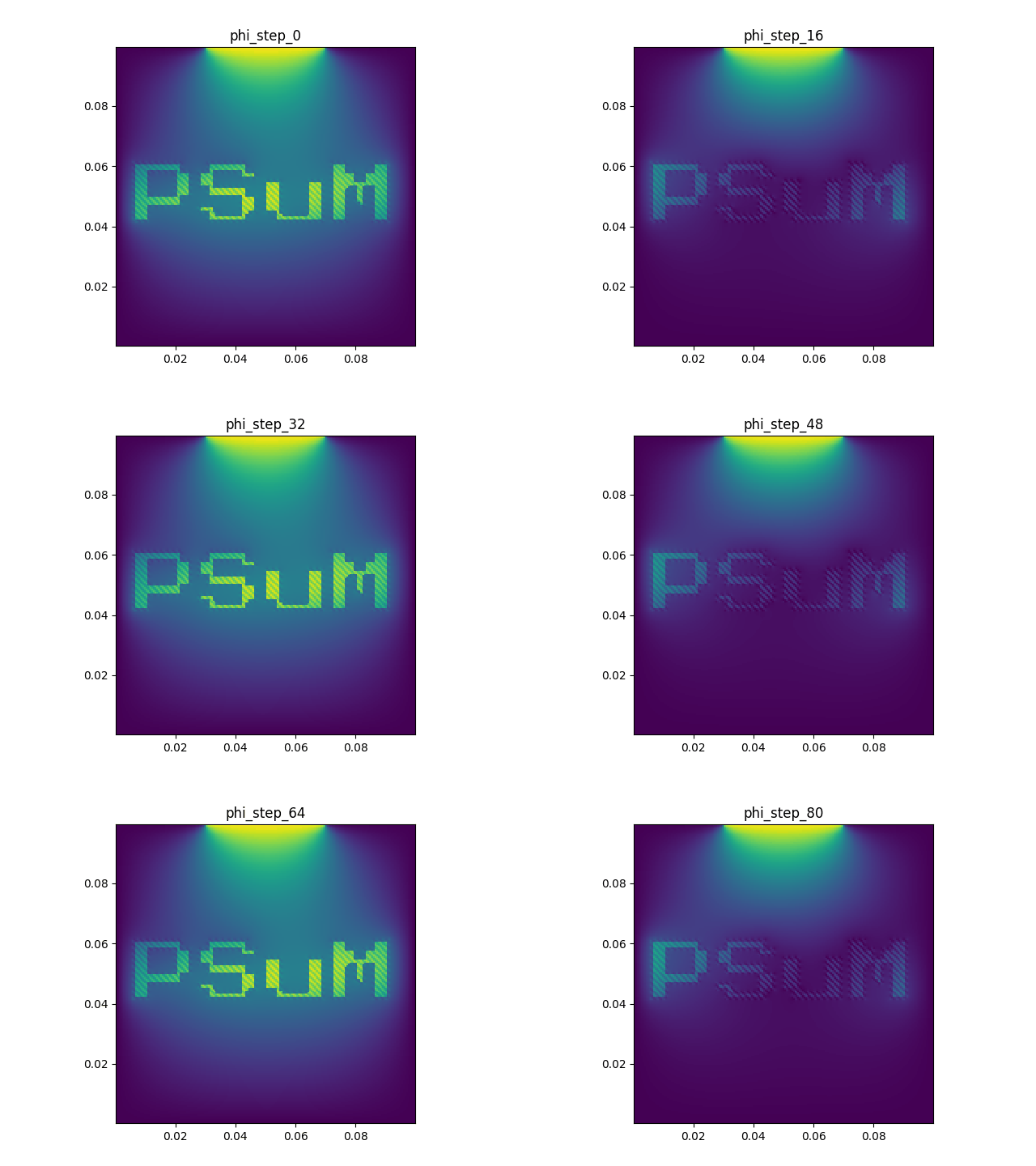
Modules, features, and typical usage covered:
- Reading external
.pltfiles - Setting complex boundaries for the 2D Poisson equation
Preparation
Create neon_light.cpp under example/neon_light/, then modify this file step by step following each stage.
example/neon_light/stage_1.cpp through stage_5.cpp are reference answers at the end of each stage, for comparison with your own code; they are not programs you need to run.
The input bitmap file is located at:
It is a 100 x 100 node field with variable name n, containing a binary pattern.
It is a text .plt file; you can open it in Tecplot by changing the extension. The unusual filename is simply to prevent git from ignoring it.
It is recommended to enter the example directory from the project root and load the build environment:
There may be leftover .plt, .png, or .gif files in output/.
You can manually clear output/ first.
Stage 1: Read the Bitmap and Restore the Node Field
In neon_light.cpp, first include the necessary headers and use the PSuM prelude:
#include <cmath>
#include <fstream>
#include <iostream>
#include <sstream>
#include <string>
#include <vector>

#include <psum/psum.hpp>

using namespace std;
using namespace psum::prelude;
Next, implement a small function to restore a PSuM .plot output point-type .plt file into a host_node_field2D<double>:
host_node_field2D<double> read_node_field_plt(const string& filename) {
    ifstream in(filename);

    string line;
    string zone;
    getline(in, line);
    getline(in, zone);

    vector<double> values;
    double xmin = 1e300;
    double xmax = -1e300;
    double ymin = 1e300;
    double ymax = -1e300;
    double x = 0.0;
    double y = 0.0;
    double v = 0.0;
    while (getline(in, line)) {
        istringstream row(line);
        if (!(row >> x >> y >> v)) {
            continue;
        }
        xmin = fmin(xmin, x);
        xmax = fmax(xmax, x);
        ymin = fmin(ymin, y);
        ymax = fmax(ymax, y);
        values.push_back(v);
    }

    int ni = stoi(zone.substr(zone.find('=', zone.find('i')) + 1));
    int nj = stoi(zone.substr(zone.find('=', zone.find('j')) + 1));

    grid2D grid({xmin, ymin}, {xmax, ymax}, {nj - 1, ni - 1});
    return host_node_field2D<double>(std::move(values), grid);
}
Note here:
- In a 2D
.pltfile,zone icorresponds to the number of nodes in the second coordinate direction, andzone jcorresponds to the number of nodes in the first coordinate direction, so when restoring thegrid2D, we use{nj - 1, ni - 1}.
In main, read the bitmap and output it immediately to verify the reading direction and pattern are correct:
int main() {
    const string bitmap_file = "../../docs/psum_tour/psum_bitmap(.plt)";
    auto mask = read_node_field_plt(bitmap_file);
    mask.plot("output/mask.plt", "mask", 0.0);
    return 0;
}
In the makefile, create output/ for this stage, run neon_light.cpp, and convert .plt to an image:
-include ../../config.mk

INCLUDES = -I ../../include -I ../../src

neon_light: neon_light.cpp
    $(ACPP) $(COMMON_FLAGS) $(INCLUDES) -o neon_light neon_light.cpp $(LIBS) $(LDFLAGS)
    mkdir -p output
    ./neon_light
    python3 ../pltview.py output/mask.plt

clean:
    rm -f neon_light
    rm -rf output
(These commands already exist in example/neon_light/makefile; just uncomment them.)
Compile and run the same way for each subsequent stage:
After a successful run, you should see output/mask.plt (open with Tecplot) and output/mask.png (viewable directly).
What you need to know at this stage:
host_node_field2D<double>is a host-side node-centered 2D field.- The
x y ndata in a.pltfile can be restored into the field's content. mask.plot(...)is used to quickly verify the read result.
The code state at the end of this stage can be found in example/neon_light/stage_1.cpp.
Stage 2: Create the Poisson Grid and Solve Once
Continue modifying neon_light.cpp from Stage 1:
- Add
using namespace psum::field_solver::boundary_creator;. - Inherit the physical range from
mask.getGrid()and create a 200 x 200 Poisson grid. - Configure Dirichlet boundaries with zero on all four sides.
- Temporarily use the mask region as a source, solve once, and output the result.
The Poisson grid can have a different resolution than the input bitmap grid. Here we use a finer 200 x 200 grid, but the physical range is inherited from the bitmap:
const auto& mask_grid = mask.getGrid();
grid2D grid(
    {mask_grid.lowerBound<0>(), mask_grid.lowerBound<1>()},
    {mask_grid.upperBound<0>(), mask_grid.upperBound<1>()},
    {200, 200}
);
Create and initialize the solver. For now, set all four edges to zero fixed-value boundaries:
Poisson_solver_2d solver;
solver.init(
    grid,
    Poisson_solver_2d::Cartesian,
    {
        Dirichlet_line(grid, boundary_direction_2d::N) = 0.0,
        Dirichlet_line(grid, boundary_direction_2d::S) = 0.0,
        Dirichlet_line(grid, boundary_direction_2d::E) = 0.0,
        Dirichlet_line(grid, boundary_direction_2d::W) = 0.0
    }
);
To verify that the solver and output pipeline work, you can set the pattern region as a source:
host_node_field2D<double> phi(grid);
host_node_field2D<double> source(grid);
source.for_each([&](size_t, double& rho, const auto& pos) {
    rho = interp(host_node_field2D<double>::Position{pos[0], pos[1]}, mask) > 0.5 ? 10.0 : 0.0;
});

solver.solve(phi.data(), source.data());
phi.plot("output/phi.plt", "phi", 0.0);
From this stage onward, you need to link the Poisson solver backend, so change the compilation line in the makefile to:
If you get compilation errors about not finding Poisson-related implementations, first confirm that $(USE_BACKENDS) has been added to the makefile.
Run:
After a successful run, you should see output/phi.plt and output/phi.png.
Compared to the mask output, the phi output looks much softer, and the pattern outline may even be hard to see. This is due to the nature of the Poisson equation.
What you need to know at this stage:
- The Poisson grid's physical range can come from an existing field.
interp(..., mask)can interpolate values between grids of different resolutions.solver.solve(phi.data(), source.data())writes the solution result intophi.
The code state at the end of this stage can be found in example/neon_light/stage_2.cpp.
Stage 3: Turn the Pattern into an Internal Dirichlet Boundary
Continue modifying neon_light.cpp from Stage 2:
- No longer use the pattern as a source.
- Use
Dirichlet_functo set the pattern region as an internal Dirichlet boundary.
The internal boundary selector function is written directly inside solver.init(...), after the existing west boundary condition:
        Dirichlet_line(grid, boundary_direction_2d::W) = 0.0,   // <-- added a comma
        Dirichlet_func(grid, [&](double x, double y) {
            return interp(host_node_field2D<double>::Position{x, y}, mask) > 0.01;
        }) = 1.5
Here we don't write a custom interpolation utility function, but instead use the interp already available in the PSuM field module.
Linear interpolation produces intermediate values between 0 and 1 at the edges of the 0-1 region, so we use 0.01 as the threshold.
At this stage, set the source to zero and only observe the potential generated by the boundary conditions:
host_node_field2D<double> phi(grid);
host_node_field2D<double> source(grid);
source.setZero();

solver.solve(phi.data(), source.data());
phi.plot("output/phi.plt", "phi", 0.0);
Run:
After a successful run, you should see output/phi.plt and output/phi.png have changed.
Compared to the previous stage's output, the entire pattern region appears to be "glowing."
What you need to know at this stage:
Dirichlet_funccan use any boolean function to select internal fixed-value regions.- The mask and Poisson grid don't need to match; the hit detection is handled by
interp. - Multiple boundary conditions can be placed in the same
solver.init(...)list.
The code state at the end of this stage can be found in example/neon_light/stage_3.cpp.
Stage 4: Make the Internal Boundary Value Change Over Time
Continue modifying neon_light.cpp from Stage 3:
- Change the internal Dirichlet value from a constant to a lambda.
- Add a time variable
t. - Add a loop to repeatedly solve and output
phi_step_*.plt. - In the makefile, combine
phi_step_*.pltinto an animation.
Before defining the solver, define a potential function that changes rapidly with time and space:
double t = 0.0;
auto voltage = [&](double time, double x, double y) {
    double high_freq = sin(3000.0 * (x + y) + 100.0 * time) + 1;
    double low_freq = cos(30.0 * (x - y) - 10.0 * time) + 1;
    return (high_freq * 0.2 + low_freq) * cos(60 * y - 3);
};
Then change the internal boundary assignment to a lambda:
Dirichlet_func(grid, [&](double x, double y) {
    return interp(host_node_field2D<double>::Position{x, y}, mask) > 0.01;
}) = [&](const auto& pos) {
    return voltage(t, pos[0], pos[1]);
},
solver.init(...) only needs to be called once.
In the subsequent loop, update t, then call solver.solve(...):
int steps = 80;
double dt = 0.02;
for (int step = 0; step <= steps; ++step) {
    t = step * dt;
    source.setZero();
    solver.solve(phi.data(), source.data());
    phi.plot("output/phi_step_" + to_string(step) + ".plt", "phi", t);
    cout << "step = " << step << ", t = " << t << endl;
}
Run:
Also adjust the plotting commands in the makefile to:
After a successful run, you should see step = ... printed in the terminal, and output/phi_step.gif generated.
What you need to know at this stage:
- The boundary value lambda captures the variable
t, so each solve step gets a different fixed-value boundary. - The dynamic effect in the animation comes from the time-varying Dirichlet boundary.
The code state at the end of this stage can be found in example/neon_light/stage_4.cpp.
Stage 5: Add Edge Weak Potential and Complete the Neon Light Effect
Continue modifying neon_light.cpp from Stage 4:
- Overlay partially selected Dirichlet boundaries.
- Use the intermediate values from linear interpolation to add a weaker edge Dirichlet boundary.
Even after boundary conditions have been set, later-set ones can override earlier ones. Add the following after the original north boundary:
        Dirichlet_line(grid, boundary_direction_2d::N) = 0.0,
        Dirichlet_line(grid, boundary_direction_2d::N,
            {grid.lowerBound<0>() + 0.3 * grid.span<0>(),
             grid.upperBound<0>() - 0.3 * grid.span<0>()}) = 2.5, // Set a higher fixed value on a short segment of the north boundary
Function-type boundary conditions can also be overlaid. Linear interpolation interp(..., mask) produces values between 0 and 1 at the edges of the mask. Select this region and place it after the original settings:
Dirichlet_func(grid, [&](double x, double y) {
    return interp(host_node_field2D<double>::Position{x, y}, mask) > 0.01;  // <-- original boundary condition
}) = [&](const auto& pos) {
    return voltage(t, pos[0], pos[1]);
},                                                                          // <-- added a comma
Dirichlet_func(grid, [&](double x, double y) {
    double mask_val = interp(host_node_field2D<double>::Position{x, y}, mask);
    return mask_val > 0.01 && mask_val < 0.99;                          // <-- select the edge of the mask
}) = [&](const auto& pos) {
    return voltage(t, pos[0], pos[1]) * 0.5;                            // <-- use a different fixed value
}
Run:
After a successful run, the final output includes:
You should be able to see a fairly clear pattern outline and a flickering effect.
What you need to know at this stage:
- Boundary conditions can be overlaid; later-set conditions override earlier ones.
- The key API path for this entire example is
read_node_field_plt,interp,Dirichlet_func, andPoisson_solver_2d.
The code state at the end of this stage can be found in example/neon_light/stage_5.cpp.
Output and Common Errors
pltview.py has two common usage patterns:
The first is for a single .plt file, typically generating a corresponding .png.
The second is for a set of files; it searches output/ for .plt files starting with rho_step_ and combines them into an animation; phi_step output and energy output work similarly.
Common errors can be investigated as follows:
make: acpp: No such file or directory: Usually means you haven't runsource ../../env_load.sh.No rule to make target 'neon_light': You're in the wrong directory, or theneon_lighttarget hasn't been added to the makefile yet.No rule to make target 'neon_light.cpp': Theneon_lighttarget exists, but you haven't createdneon_light.cppin the current directory yet.- No
output/...files generated: Confirm the makefile hasmkdir -p output, and that the program is running underexample/neon_light/. pltview.pydoesn't printwrote ...: The plotting script didn't complete successfully; check the Python error output above in the terminal.- Linker error about missing backend
.ofiles: Build the field solver backend first, or check whether the backends enabled inconfig.mk.localmatch your local environment. - Seeing
AdaptiveCpp Warning: These are usually runtime JIT compilation hints and not necessarily program errors; as long as the program continues to output and generate files, everything is fine.